
The Complete Solution to $\bf{A}\bf{x}=\bf{b}$
A Flowchart (with commentary) to derive the solution types for a system of linear equations.
I was revisiting some linear algebra basics and could not find a good resource that put together all the scenarios in which the various solution types of $\bf{A}\bf{x}=\bf{b}$ ocurred. The flowchart and explanation that follows is my attempt at covering all the bases. I assume the reader has a basic understanding of linear algebra. Here’s a good refresher if you need one.
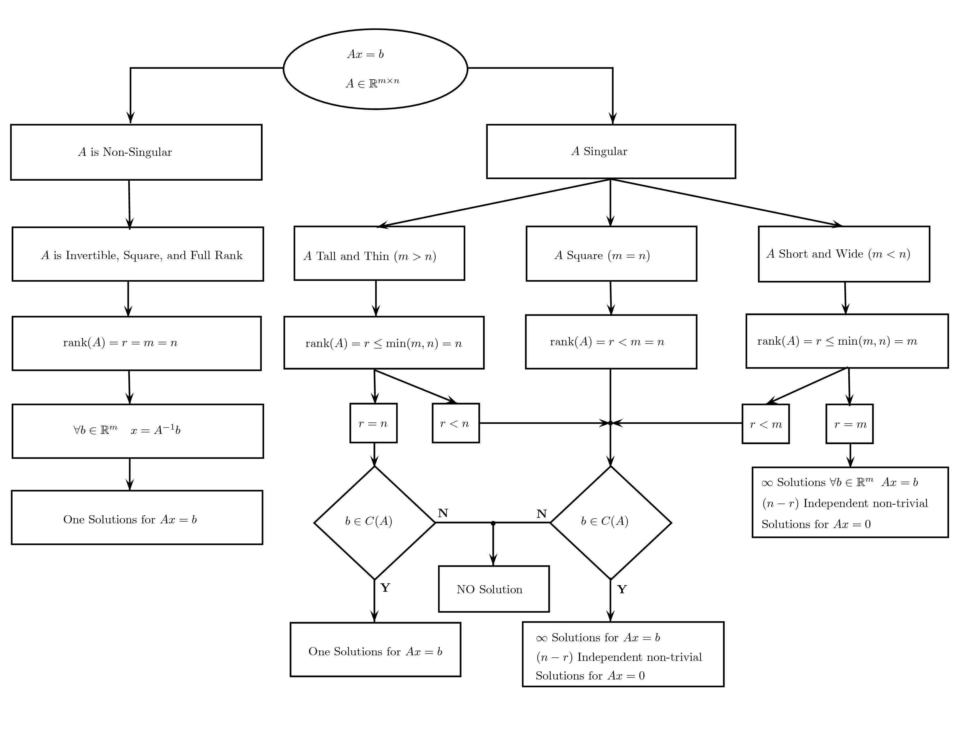 The above flowchart presents the train-of-thought along with the core concepts needed to derive a solution type from the structure of $\bf A$.
For better viewing, click the image to open in a new tab.
Notations
- $\mathbf{A} \in \mathbb{R}^{m\times n},\;\;\mathbf{x}\in \mathbb{R}^{n},\;\;\mathbf{b}\in \mathbb{R}^{m}$.[1]
- $C(\mathbf{A})$ denotes the Column Space of $\bf A$. When the matrix is represented as a linear transformation, it is also know as the Image of $\bf A$, denoted by $Im(\mathbf{A})$.
- $dim(V)$ denotes the dimension of a vector space $V$. It is the cardinality of a basis set of $V$.
- $r := rank(\mathbf{A})$ is the rank of matrix $\bf A$. Loosely speaking, rank is the number of linearly independent columns of the matrix.
[1]: We chose the matrix to be defined over the reals to keep things simple. The details in the post are applicable to matrices defined over any field.
Different Solution Types
The solution types for $\bf{A}\bf{x}=\bf{b}$ falls into three categories.
- No Solution: There is no linear combination of the columns of $\bf A$ that can produce a specific $\bf b$, i.e. $\mathbf{b} \not\in C(\mathbf{A})$
- One Solution: All the columns of $\bf A$ form a linearly independent set, and $\mathbf{b} \in C(\mathbf{A})$
- $\infty$ Solutions: $\bf b$ can be formed as the linear combination of more that one set of linearly independent columns in $\bf A$.
One natural question to ask is, could there be more than one but less than infinite solutions. The answer is no. Theorem 1 in the Appendix section gives a constructive proof.
Complete Solution
We start by looking at the invertibility of $\bf A$. $\bf A$ is invertible if it is full rank and square. A matrix is considered to have full rank when $r=\min\{m, n\}$. A useful result about rank that we use in this post is $r\leq\min\{m, n\}$. A simple proof is given as Theorem 2 in the Appendix.
$\mathbf{A}$ is invertible
Let $\mathbf{A}$ be invertible, then we have the following observations.
- $\mathbf{A}$ has full rank, hence all the columns are linearly independent and span $\mathbb{R}^m$
- $\forall\mathbf{b}\in\mathbb{R}^{m}\;\;\mathbf{b}\in C(\mathbf{A})$
- Therefore we have exactly one solution for $\bf{A}\bf{x}=\bf{b}$, given by $$\mathbf{x} = \mathbf{A^{-1}b}$$
$\mathbf{A}$ is singular
Let $\mathbf{A}$ be singular, i.e. non-invertible. Here we have three possibilities based on the shape of $\mathbf{A}$.
- Tall and Thin $(m>n)$: Since $r\leq \min\{m, n\}=n$, we have two options.
- $(r=n)$: All the columns of $\bf A$ are linearly independent and they span an $n$-dimensional subspace of $\mathbb{R}^m$. If $\bf b$ lies inside this subspace, we have a solution for $\bf{A}\bf{x}=\bf{b}$, otherwise there is no solution. If we have a solution, then there is only one linear combination of the columns of $\bf A$ that gives a specific $\bf b$. Hence, there is only one solution.
- $(r<n)$: $\bf A$ is not full rank, only $r$ columns are linearly independent. Similar to the above case, if $\bf b$ lies in the $r$-dimensional subspace, we have a solution, otherwise no solution.
The remaining $(n-r)$ columns are some linear combination of the others. A result shows that these $(n-r)$ columns induce $(n-r)$ independent solutions to the equation $\bf A\bf x = \bf 0$. The proof is an involved one, a good explanation can be found here. Let $\mathbf{x}_n$ be one such solution to $\bf A\bf x = \bf 0$, and let $\mathbf{x}_p$ be the solution to $\bf{A}\bf{x}=\bf{b}$. That is, \begin{align} \mathbf{A}\mathbf{x}_n & = \mathbf{0} \\ \mathbf{A}\mathbf{x}_p & = \mathbf{b} \\ \therefore \mathbf{A}(\mathbf{x}_n+ \mathbf{x}_p) & = \bf b \end{align} Hence $(\mathbf{x}_n+ \mathbf{x}_p)$ is also a solution to $\bf{A}\bf{x}=\bf{b}$. Now since we have two solutions, $\bf{A}\bf{x}=\bf{b}$ has infinite solutions (Theorem 1, Appendix).
- Square $(m = n)$: When a matrix is square and singular it is not full rank. Hence $(r < m = n)$, which is same as the $(r < n)$ scenario when the matrix was tall and thin.
- Short and Wide $(m < n)$: Since $r\leq \min\{m, n\} = m$, we have two options.
- $(r<m)$: $(r < m < n) \rightarrow (r < n)$. Hence, this scenario is the same as $(r < n)$ when the matrix was tall and thin.
- $(r=m)$: A remarkable non-intuitive theorem in linear algebra states that the row rank and the column rank of a matrix $\bf A$ are equal. Row rank is the number of linearly independent rows, and the column rank is the number of linearly independent columns. Proofs for this theorem can found on wikipedia.
Using the theorem, the number of linearly independent columns of $\bf A$ is $m$, and hence it spans the whole of $\mathbb{R}^{m}$. Therefore, $\forall\mathbf{b}\in\mathbb{R}^{m}$ we have a solution for $\bf{A}\bf{x}=\bf{b}$.
Similar to the $(r < n)$ case when the matrix was tall and thin, there is $(n-m)$ independent solutions to $\bf A\bf x = \bf 0$. Therefore, $\bf{A}\bf{x}=\bf{b}$ has infinite solutions $\forall\mathbf{b}\in\mathbb{R}^{m}$.
Thats it, we’ve covered the solution types for $\bf{A}\bf{x}=\bf{b}$ based on all the possible structure $\bf A$ can take.
Appendix
Theorem 1. A system of linear equations given by $\bf{A}\bf{x}=\bf{b}$ cannot have more than one but less than infinite solutions.
Proof. Assume that $\bf{A}\bf{x}=\bf{b}$ has two solutions $\bf u$ and $\bf v$. Now consider the line that passes through both the points. $$\theta\mathbf{u} + (1-\theta)\mathbf{v} \qquad\forall\theta\in\mathbb{R}$$ Without loss of generality, consider an instantiation of $\theta$, say $\theta_1$. Let $\bf w$ be the point on the line such that, $$\mathbf{w} = \theta_1\mathbf{u} + (1-\theta_1)\mathbf{v}$$ Left multiply both sides with $\bf A$, we get $$\mathbf{A}\mathbf{w} = \theta_1\mathbf{A}\mathbf{u} + (1-\theta_1)\mathbf{A}\mathbf{v}$$ Now since $\bf u$ and $\bf v$ are solutions of $\bf{A}\bf{x}=\bf{b}$, we have, \begin{align} \mathbf{A}\mathbf{w} & = \theta_1 \mathbf{b} + (1-\theta_1)\mathbf{b} \\ & = \mathbf{b} \end{align} Clearly $\mathbf{w}$ is also a solution for $\bf{A}\bf{x}=\bf{b}$. Moreover, since $\theta_1$ was arbitrarily chosen, $\forall\theta\in\mathbb{R}\quad\theta\mathbf{u} + (1-\theta)\mathbf{v}$ is a solution for $\bf{A}\bf{x}=\bf{b}$. Therefore, if there exists more than one solution, then $\bf{A}\bf{x}=\bf{b}$ necessarily has infinitely many solutions.$\;\;\small\blacksquare$
Theorem 2. Given any matrix $\mathbf{A}\in\mathbb{R}^{m\times n}$, the following inequality holds. $$rank(\mathbf{A})\leq\min\{m, n\}$$
Proof. We defined rank as the number of linearly independent columns of $\bf{A}$, $$\therefore rank(\mathbf{A})\leq n \tag{1}$$ The matrix $\bf A$ can be considered as the linear transformation $$\mathbf{A}:\mathbb{R}^n\rightarrow\mathbb{R}^m$$ Therefore, the space spanned by the image of $\bf A$ is a subspace of $\mathbb{R}^m$. A basis for this subspace is the linearly independent columns of $\bf A$. Hence, \begin{align} rank(\mathbf{A}) & = dim(Im(A)) \\ & \leq m \tag{2}\end{align} From $(1)$ and $(2)$ we get, $$rank(\mathbf{A}) \leq \min\{m, n\}$$ $\;\;\small\blacksquare$
I like blocks and arrows, it lends perspective to where you come from and where you go.

