Introduction

More often than not, the difference between a crappy and powerful implementation of a Machine Learning (ML) algorithm is the choice of its hyperparameters. Hyperparameter Tuning was considered an artistic skill that ML practitioners acquired with experience. Over the past few years several advancements have been made in this area to perform hyperparameter tuning in a more informed manner. Techniques such as Bayesian Optimization, Neural Architecture Search, Probabilistic Matrix Factorization have been developed in the recent past to tackle hyperparameter tuning with great success. In a series of posts we try to understand the theory behind Bayesian Optimization (BO) and then provide an implementation for a toy problem. For a case study on the efficacy of BO in a production setting the paper Chen et al. (2018) from Deepmind provides a detailed account on how they used BO to tune the hyperparameters of AlphaGo.

In this part we discuss Stochastic Processes, a crucial mathematical building block that can model noise in physical systems. Later in Part-2 we’ll discuss Gaussian Process, and finally in Part-3 we’ll introduce Bayesian Optimization along with a toy implementation.

This post assumes that the reader has a basic knowledge in probability and statistics.

Random Variables

Random Variables (RV) are deterministic functions that maps all possible outcomes of a probabilistic experiment to some mathematical space, like $\mathbb{R}$, on which analysis is possible. Roughly speaking, the idea is to obtain numerical outcomes for experiments whose outcomes may not be numerical, such as mapping Heads to $1$ and Tails to $0$ in a coin toss experiment. A numerical representation allows us to perform further analysis on the experiment such as evaluating central tendencies, performing inference etc. The name Random Variable is unfortunate as the randomness and variability is characteristic of the underlying experiment, rather than the function itself. Let’s start by defining it more formally.

Definition 1 (Probability Space). For some probabilistic experiment, let $\Omega$, called the sample space, denote the set of all possible outcomes for the experiment. Let $\mathcal{F}$, called the $\sigma$-algebra(event space), denote a collection of subsets of $\Omega$, and let $P: \mathcal{F} \rightarrow [0,1]$, called the probability measure, be a function that assigns to each element in $\mathcal{F}$ a value between $[0,1]$ that is consistent with the axioms of probability. Then the triplet $(\Omega, \mathcal{F}, P)$ is called a probability space.

Example (Fair Coin Toss). Given an experiment where we toss a fair coin the probability space $(\Omega, \mathcal{F}, P)$ is as follows:

• $\Omega = \{H, T\}$

• $\mathcal{F} = \mathcal{P}(\Omega) = \{\emptyset, \{H\}, \{T\}, \{H, T\}\}$

• $P(\emptyset) = 0, P(\{H\}) = 0.5, P(\{T\}) = 0.5, P(\{H, T\}) = 1$

Definition 2 (Random Variable). Given a probability space $(\Omega, \mathcal{F}, P)$, a Random Variable $X$ is a function from $\Omega$ to a measurable space $E$. That is, $$X: \Omega \rightarrow E\qquad$$

Roughly, a measurable space can be thought of as the set on which mathematical analysis is possible. The real-line, $\mathbb{R}$, is an example of a measurable space. When $E=\mathbb{R}$ in the above definition, the RV is called a real-valued random variable. Real-valued RVs are the most common and is widely used in statistics to quantify properties such as central tendencies, moments, CDF, etc. of a distribution.

Discrete and Continuous Random Variables

If the image of $X$ is countable then $X$ is a discrete random variable, and its distribution is defined by a probability mass function. On the other hand, if the image of $X$ is uncountable, then $X$ is a continuous random variable, and its distribution may be defined by a probability density function ¹. To really flush out the differences between discrete and continuous RVs we need to invoke more measure theoretic aspects, which is irrelevant in the context of this post.

Stochastic Process

A Stochastic Process a.k.a. Random Process is a mathematical object that represents a collection of Random Variables. The word process, which means “something that is a function of time”, is used in the name because stochastic processes were primarily employed for investigating the evolution of probabilistic systems over time. Generally, the process need not have anything to do with time.

For example, a general procedure to study the properties of a probabilistic system is to run experiments that collect samples as the system evolves through time. Once the experiment is finished, the system is reset to initial conditions and the same experiment is run multiple times so as to study the variability in the system. Each experiment run gives a sample path (a.k.a. sample realization or sample function) for the time-evolution of the system. The sample path can be modelled as a sequence of random variables, $X_1 = (Y_1, Y_2, \ldots)$, and the entire process can then be modelled as a family of random sequences $X=\{X_1, X_2, \ldots X_n\}$. Say, if $\Omega = \{1,\ldots, n\}$, and $Y_i$ is a real-valued random variable, then $X$ is a mapping from $\Omega$ to the space of real-valued discrete functions. For example, $X(1)$ gives you the discrete function $(Y_1, Y_2, \ldots)$. At the same time, $X$ is also a collection of random variables as it’s a family of random sequences. See Figure-1 for a visualization of the process.

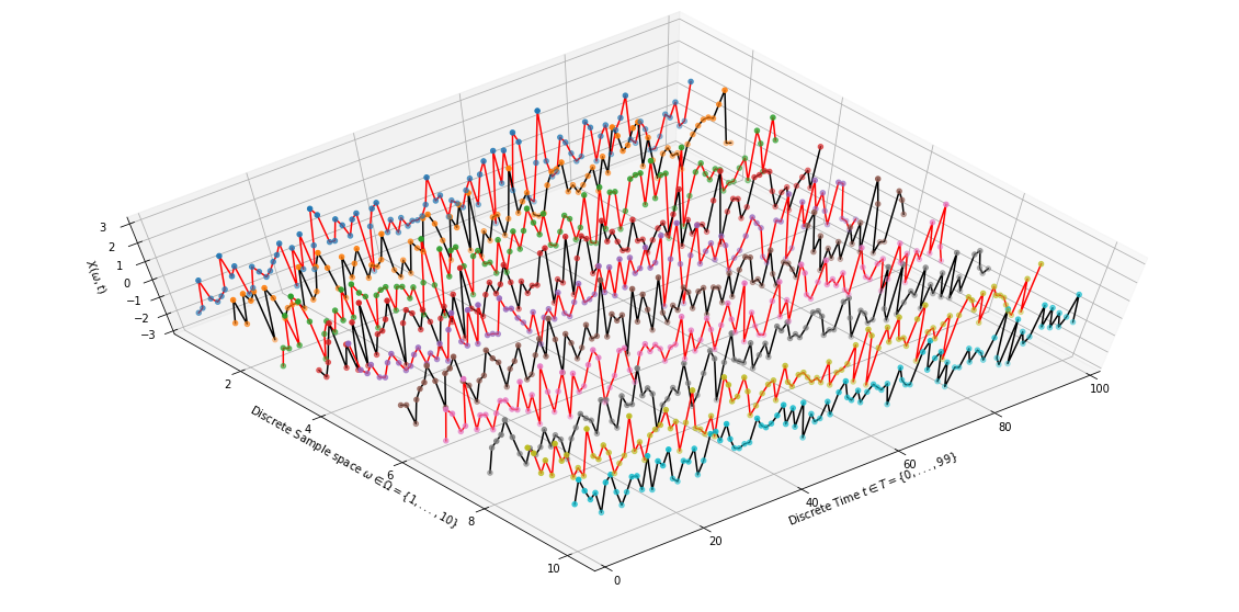
Figure 1: A Discrete-time Stochastic Process (Samples are connected for visualization)

Let’s define it formally,

Definition 3 (Stochastic Process). Given a probability space $(\Omega, \mathcal{F}, P)$, a Stochastic Process, $X$ is both a collection of Random Variables all taking values in the same measurable space $E$, as well as a mapping from the sample space $\Omega$ to a space of functions.

When $X$ is represented as a collection indexed by a set $T$, it can be written as, $$X = \{X_t : t\in T\}\quad where\,\, X_t \text{ is an }E\text{-valued r.v.}$$Alternatively, when $X$ is represented as a mapping to a space of functions, it can be written as, $$X: \Omega \rightarrow E^{T}$$

Depending on the nature of the underlying probability system there are different kinds of stochastic processes. For instance, if the system emits a continuous signal then the stochastic process is modelled with an uncountable index set making it a continuous stochastic process. On the other hand, if the samples are taken at discrete intervals then the index set is countable, making the process discrete. We can use the various aspects of the process and the underlying system to model different kinds of stochastic processes. Rather than listing them out, let’s focus on the key aspects of a stochastic process to get a broader picture.

Index Set

The set that is used to index the RVs in a stochastic process is called an index set. The index set, $T$, is any valid mathematical set, but it is preferred that $T$ be linearly ordered so as to enable further analysis. When $T$ is countable, like $\mathbb{N}$ or $\{1,\ldots, N\}$, the random process is said to be discrete, and is often called a Discrete-time Random Process. On the other hand, when $T$ is uncountable, like $\mathbb{R}$ or $[0,1]$, the random process is said to be continuous and is often called a Continuous-time Random Process.

State Space

The state space of a random process is the values that the RVs in the collection can take. The word state-space is so designed to evoke the notion that random process as a whole has a current state and can move to different states as time progresses. Interpreting the index set as time, the current state of the random process is the value of the random variable $X_t$, where $t$ is the time elapsed since start of the experiment. The state space is discrete if it is countable, and the process is called discrete-valued stochastic process. Similarly, the state space is continuous if it is uncountable, and the process is called a continuous-valued stochastic process.

Stationarity

If all the random variables in a stochastic process is identically distributed then the process is said to be stationary, i.e. the distribution of the system from which we are sampling does not change over time. A simple example of a stationary random process is the Bernoulli process.

Alternate View of a Stochastic Process

For the purposes of our analysis in the the context of Bayesian Optimization we want to look at stochastic processes from a probabilistic view point. From the definition we know that sampling a stochastic process gives us a function. Thus, a stochastic process can also be represented as a probability distribution over a space of functions, and sampling from this distribution gives you a sample realization of the process.

When $X$ in finite, $P(X)$ can be described as the joint distribution $P(X_1,X_2,\ldots, X_n)$ for some finite $n$, called the finite-dimensional distribution. When $X$ is countably infinite or uncountable, which is most of the time, things become complex as $P(X)$ becomes an infinite-dimensional distribution. Even though not technically correct, to keep things simple, just think of the stochastic process as the joint distribution over all the random variables in the collection, and that a sample from this distribution is a time-dependent function. That is, $$f(t) \sim P(X_1, X_2, \ldots)$$

Examples

Bernoulli Process

Let $X_t$ be a random variable defines as, $$X_t=\begin{cases} 1 & w.p.\,\, p \\
0 & w.p.\,\, 1-p \end{cases}$$ for some fixed $p$. $X_t$ is called a Bernoulli random variable. The sequence of independent and identically distributed (i.e. with same $p$) Bernoulli random variables, $X=\{X_0, X_1, \ldots\}$ is called a Bernoulli Process.

Simple Random Walk

Let $Y_i$ be a random variable defined as $$Y_i=\begin{cases} s & w.p. \frac{1}{2} \\
-s & w.p. \frac{1}{2} \end{cases}$$ for some fixed $s$. Also, let $X_t$ be a random variable defined as $$X_t=\begin{cases} 0 & \text{if } t=0 \\
\sum_0^t Y_i & \text{otherwise} \end{cases}$$ The sequence of random variables $X = \{X_0, X_1, \ldots\}$ is a stochastic process called a simple random walk. Sample realizations are shown in Figure-2 for $s=1$.

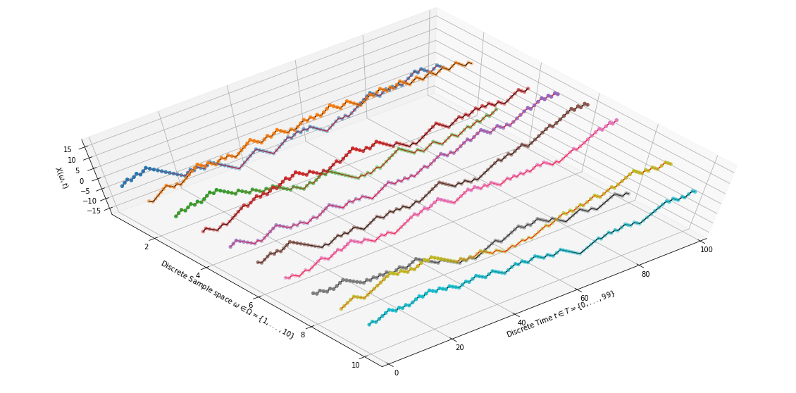
Figure 2: Sample realizations of Random Walk Process $(s=1)$

Brownian Motion a.k.a. Wiener Process.

A Brownian motion is a continuous-time version of a random walk process. Since the time is continuous we don’t have the notion of a time-step anymore, rather we talk about the increment over a fixed interval of time. The Brownian Motion $B_t$ has the following properties:

1. Independence of Increments: Given an interval $\Delta t$, $\forall s<t\,\,(B_{t+ \Delta t} - B_t) \perp B_s$

2. Normally Distributed Increments: $(B_{t+ \Delta t} - B_t) \sim \mathcal{N}(0, \Delta t)$ (i.e. Stationary Increments)

3. Continuity: $B_t$ is continuous in $t$.

Figure-3 shows sample paths from a Wiener Process with $B_0 = 0$.

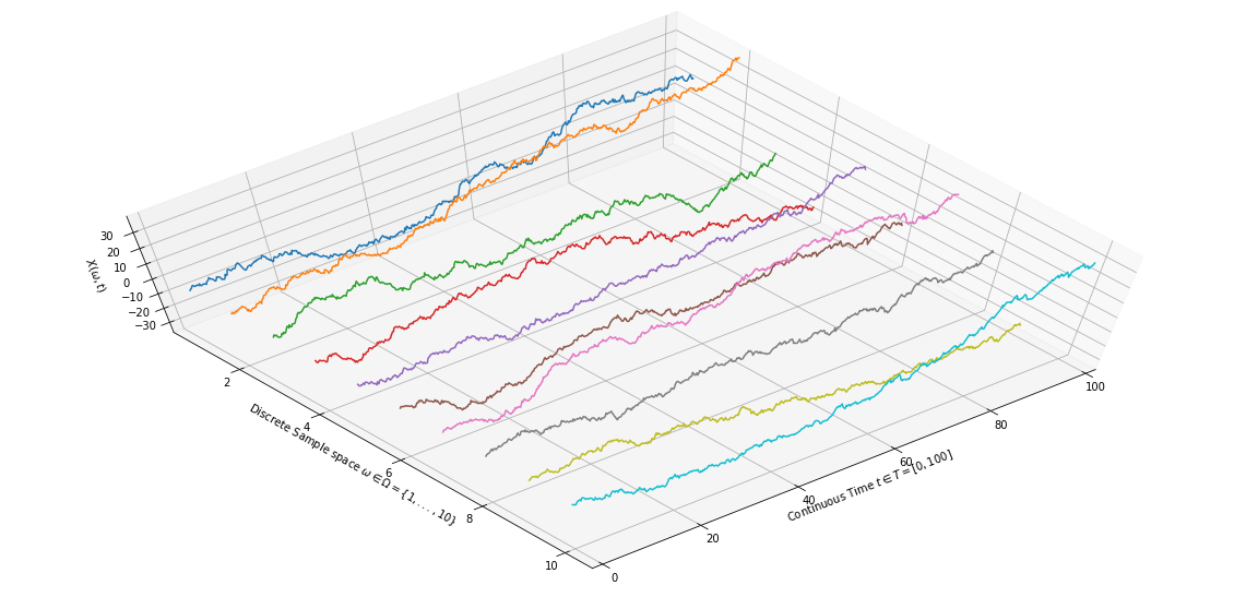
Figure 3: Sample realizations of the Wiener Process $(B_0=0)$

Conclusion

To understand Gaussian Processes and Bayesian Optimization the key takeaway from stochastic processes are the following points:

• A stochastic process is a collection of random variable

• It can also be viewed as a probability distribution over a space of functions

• Sampling a stochastic process gives a you a function which is a single time-dependent realization of the process.

In Part-2 we’ll look at Gaussian Processes in detail.